The life cycle assessment and multi-objective optimization are based on the same material inventories, environmental indicators, and cost parameters across all integration scenarios. By keeping the LCA inputs and optimization objectives unchanged, the analysis ensures that differences between scenarios are solely attributable to the maintenance integration alternatives rather than to variations in environmental or economic assumptions.
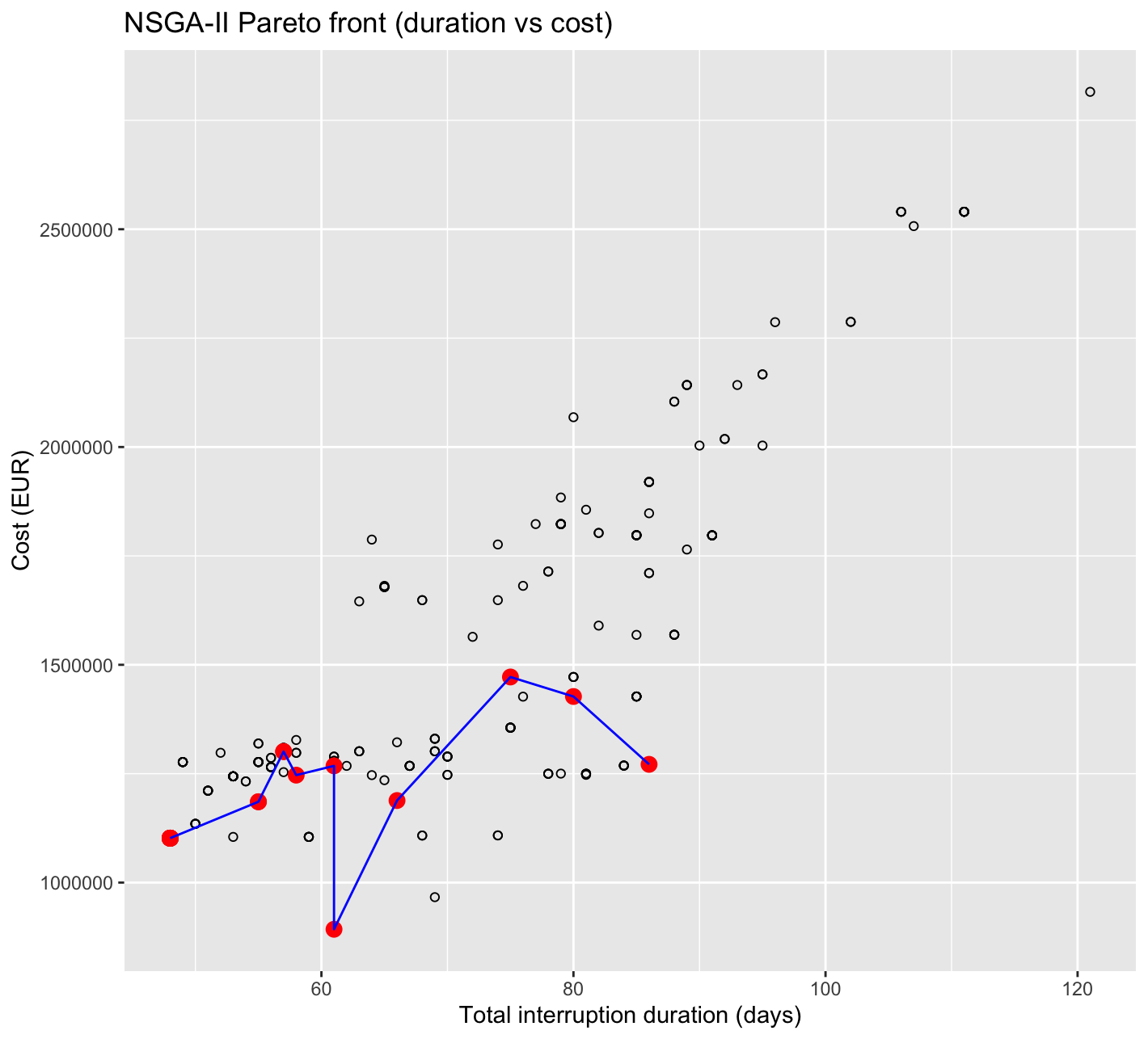
When considering the subset of more than 150 alternatives generated in the previous step, the resulting distribution in figure 2.c shows a pattern broadly similar to that observed in the first strategy. In general, an increase in the frequency of maintenance interventions leads to higher system interruption levels, which in turn results in increased overall system costs. However, unlike a smooth and monotonic Pareto trend, the Pareto front in this scenario exhibits a more fragmented and locally fluctuating structure. This behavior indicates that the proposed approach produces a more heterogeneous set of cost interruption combinations.
The main reason for this heterogeneity lies in the reorganization of maintenance interventions in terms of their content and material intensity, which allows for a wider variety of intervention combinations. In addition, it can be observed that solutions corresponding to lower total interruption durations are clustered within a relatively narrow cost band. This suggests that, at low interruption levels, different maintenance organizations can converge to similar total costs, indicating the presence of cost stabilized solution regions.
Another notable observation is that the Pareto optimal solutions in this scenario are more widely distributed in the lower left region of the Pareto space. Given that both optimization objectives explicitly aim to minimize interruption duration and cost, this distribution represents a rational outcome and provides decision makers with greater flexibility to choose among alternative maintenance organizations with comparable performance levels.
However, two distinct outliers appear around the 60 day interruption range, where abrupt cost variations can be observed. Such jumps highlight that time based performance indicators and cost based indicators do not always evolve in parallel, and that the nature of the maintenance activity itself plays a critical role. More specifically, some high cost interventions may require shorter execution times compared to lower cost activities, leading to these non intuitive combinations. This effect is particularly evident in scenarios involving gravity retaining walls, where replacement activities, despite being more expensive, can be completed in a shorter duration than certain major repair interventions.
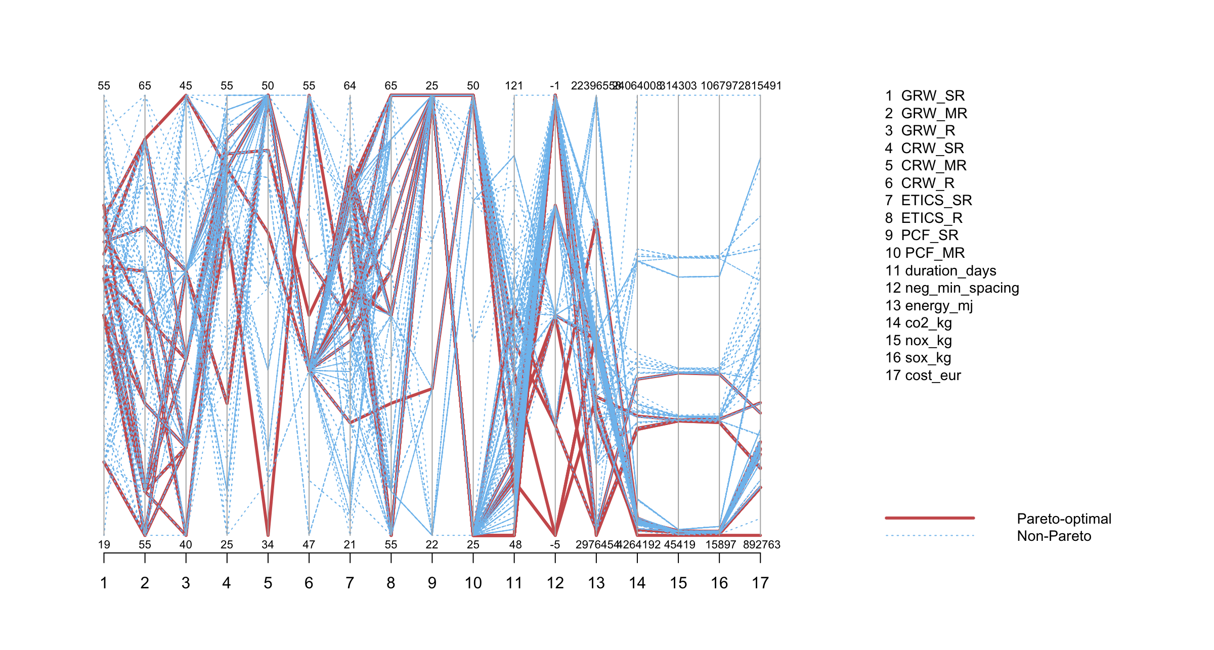
When the graph in figure 2.d is examined overall, it can be clearly observed that although Pareto optimal scenarios may approach relatively extreme values in certain criteria, they concentrate within a narrower, more consistent, and balanced band across multiple criteria, whereas non-Pareto scenarios tend to diverge toward extreme values along one or more axes. The main reason for this behavior is that Pareto optimal solutions aim to achieve balanced system level performance rather than excessively improving a single performance metric. It should be noted that overoptimizing one system output often leads to negative impacts on other system outputs. This observation is further supported by the largely parallel behavior of the life cycle assessment outputs obtained in the study. In particular, energy, emission, and cost indicators show that Pareto optimal solutions cluster near lower values without shifting toward extreme minima. In addition, although some non-Pareto alternatives cluster at relatively low values in terms of cost, emissions, and energy, they were not considered suitable alternatives because they are not optimal with respect to the time intervals between maintenance activities.
When the overall behavior of the alternatives is evaluated, it can be seen that one scenario achieves the lowest emission and cost values despite not exhibiting the best energy performance. This indicates that even with a relatively moderate level of energy consumption, the selected maintenance types and material composition can be significantly more efficient in terms of emissions and cost.
When the second and third maintenance activities those that allow alternatives to approach lower bound values along specific axes are examined in more detail, it can be observed that these maintenance types, defined for the gravity type retaining wall, have narrower allowable maintenance ranges compared to the other activities. This characteristic may have caused the solution space to shift toward these regions, as the system explores extreme values permitted within the defined constraints rather than balanced or average solutions. A similar behavior can also be observed in the ninth and tenth axes associated with the prefabricated frame system. Apart from these cases, the system generally tends to generate solutions around average values for most maintenance alternatives, indicating that only specific activities with tighter bounds drive the clustering toward extreme regions of the decision space.
When the first and second strategies and their corresponding parallel coordinates diagrams are compared, it can be observed that in both scenarios the Pareto optimal solutions tend to converge toward a specific balanced region within the multicriteria decision space. This indicates that, despite different strategic starting points, the optimization process consistently guides the system toward system level trade off solutions. However, an important difference can be identified in the shape of the Pareto front. In the second scenario, the Pareto front exhibits a more fragmented and zigzag structure compared to the first scenario. This behavior should not be interpreted as system instability, but rather as a consequence of the second strategy allowing wider ranges for some maintenance activities while imposing narrower ranges for others. In contrast, the first scenario was based on more homogeneous ranges across all activities, which resulted in a smoother and more uniform solution structure. While maintenance activities in the first scenario were grouped in a more homogeneous manner, the second scenario enables similar performance levels to be achieved through a wider variety of maintenance organizations. As a result, although the overall system behavior remains comparable in both scenarios, the decision space in the second scenario becomes slightly broader, offering the decisionmaker one or two additional feasible alternatives at similar performance levels.
An additional difference can be observed in the relationship between emissions and cost. In the first scenario, alternatives with different but parallel emission levels were found to converge to similar cost values. In the second scenario, however, alternatives with similar emission levels may exhibit more clearly diverging cost values. This can be explained by the fact that material related emission and cost values are not always directly correlated and may vary depending on the specific subsystem and material composition involved. Consequently, similar environmental impacts do not necessarily imply similar costs at the system level.
Home | System Definition | Scenario 1 | Scenario 2 | Scenario 3 | Scenario 4 | Discussion | Appendix