Multi-Objective Optimisation Analysis
Multi-objective optimisation is essential for infrastructure maintenance management as it allows us to balance competing priorities that cannot be viewed in isolation. While the Life Cycle Assessment (LCA) provided a baseline for environmental impacts and cost, the following optimisation incorporates the trade-offs between financial expenditure, environmental burdens, and serviceability metrics such as the duration and frequency of maintenance interventions. By analysing these criteria simultaneously, we can identify maintenance schedules that satisfy both Europe’s decarbonisation goal [1] and budgetary constraints.
Pareto Front: Maintenance Duration vs. Cost
The optimisation process focuses on two primary objectives: total system downtime (duration of interruptions) and total life-cycle cost. The following insights detail the trade-offs, strategic findings, and the final selection for the station’s maintenance plan.
Duration vs. Cost Trade-off: The most time-efficient alternative results in a total interruption duration of 471 days, whereas the most cost-effective alternative extends downtime to 660 days.
Cost Benefits and Investment: Despite the significant 189-day difference in duration, the cost variance is only €220,927 (0.29%). Whether this difference is considered high depends on the specific budget capabilities of the transport administration. However, the results suggest that substantial reductions in system downtime can be achieved with a relatively small increase in financial investment.
Synchronisation Strategy: The strategy achieving the minimum duration is characterised by aligning lower-frequency events to occur in the same year as planned higher-frequency interventions.
Synchronisation Costs: If reducing the duration of interventions is the goal, bundling interventions is the solution. However, at a certain point, this approach produces higher costs due to low-frequency interventions repeated more frequently than in other alternatives.
Serviceability Planning Challenges: The cost-optimised version chooses the renewal of both railway systems one year away. This represents a challenge in the planning of these projects to reduce the station shutdown.
Selected Option: With 456 days of downtime duration and a cost of € 4.568.344, the selected option finds an intermediary place between the cost and time optimised options.
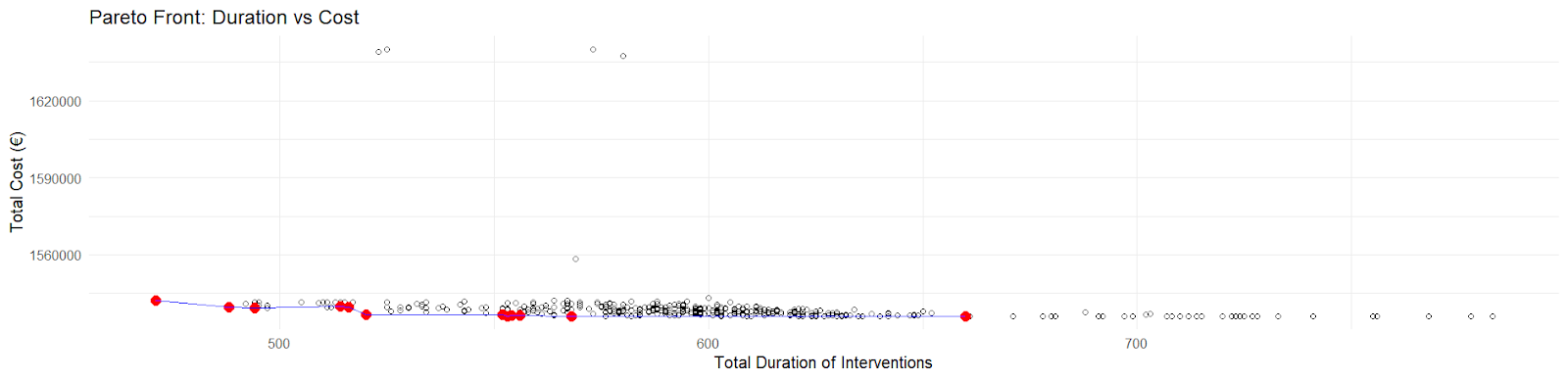
Figure 1 – Pareto front- On the under left section, the selected option.
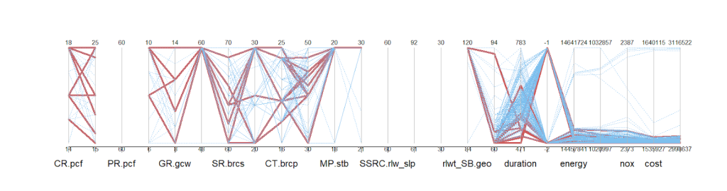
*The missing labels on the result side are the intervention’s distance, CO2 and Total Costs, respectively.
Comments on the Graphs
Figure 1 shows the Pareto Front exhibiting a scale in which it is difficult to visualise its curvature. Despite this, the trend is clear: costs increase as the search moves towards duration-optimised alternatives. The points in the higher cost area, which create this specific scale, are a direct reflection of the alternatives represented by the blue lines in Figure 2.
When visualising the intervention selection as displayed in Figure 2, it is evident that there is convergence toward a specific cost region. The blue lines suggest that the optimisation algorithm evaluated alternatives that, even when being similar to the Pareto Front selected, resulted in considerably higher costs.
Environmental Costs
The relationship between economic expenditure and ecological impact was assessed to identify the primary drivers of sustainability within the maintenance schedule.
- Environmental Cost Drivers: Energy consumption and CO2 emissions are the primary determinants of environmental costs.
- Optimal Alignment: The analysis shows a direct correlation between financial and environmental performance, as the most cost-effective solution also produced the lowest CO2 emissions.
- Carbon Pricing Relevance: The alignment of financial and environmental optimums underscores the critical impact of emission-related financial assignments on the optimisation process.
Strategies: Performance-related insights
The evaluation of the maintenance strategies revealed several key patterns regarding how interventions are scheduled over the 120 year lifecycle:
- Strategy Convergence: Highly frequent events with intervals of less than 14 years showed minimal variability, with a maximum deviation of only 2 years across all top alternatives. This suggests that optimal strategies naturally converge for routine maintenance, whereas greater differentiation occurs in long-cycle tasks.
- Frequency Range Performance for Frequent Interventions: No single frequency range (minimum, maximum, or intermediary) was favoured among the different alternatives. Top-performing solutions successfully integrated interventions across the entire admissible range to achieve a balanced schedule.
- Frequency Range Performance for Low-Frequency Interventions: For long-cycle activities, there was a clear preference for values at the higher end of the admissible range. This indicates a strategic preference to minimise the total number of times these major interventions are performed throughout the station’s lifetime.
- Distance between Interventions: Due to the high volume of required tasks, lower-frequency interventions often occurred simultaneously or in close proximity to others. Across the various optimised solutions, the longest gap between interventions was found to be only 3 years.
Algorithm Efficiency
The genetic algorithm utilised a population size of 600 across 60 generations. During the experimentation phase, various parameter sets were tested to determine if a more complex search would yield better results. Findings indicated that while increasing complexity provided a more diverse search space, the marginal gains in cost optimisation did not justify the considerable increase in simulation runtime. This outcome is visualised in Figure 3, the first graph of which displays the algorithm achieving convergence within two specific regions.
| Generations Number | Population Size | Total Costs | Percentage Variation |
| 60 | 600 | 2.998.637 | 0% |
| 80 | 800 | 2.998.637 |
Interestingly, when parameters were increased to 80 generations and a population size of 800, the effect of non-convexity was confirmed (see Figure 4). This expanded search revealed a new solution region where downtime duration was superior to that found in the initial exploration. However, this new region was not explored further in this study due to time constraints.
From a decision-making perspective, it may not be necessary to prioritise the reduction of downtime duration if it induces a higher frequency of interventions. The existing solutions have already demonstrated a balance between cost, environmental impact, and station availability.
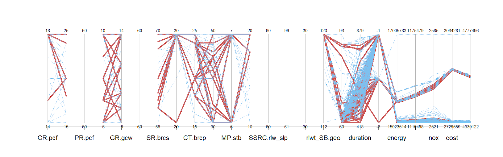
Generations: 20, Population Size: 200.
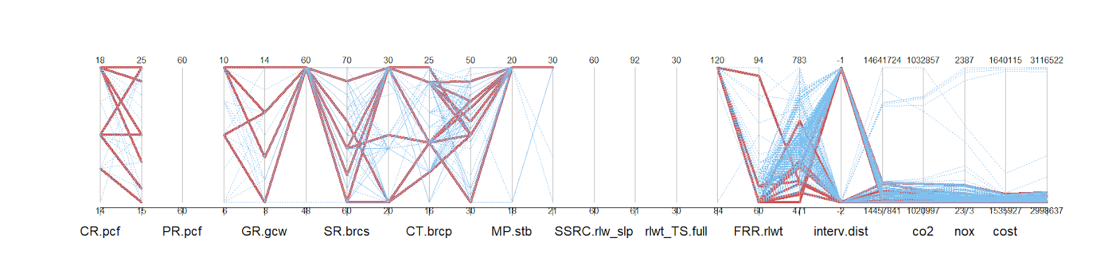
Generations: 60, Population Size: 600.
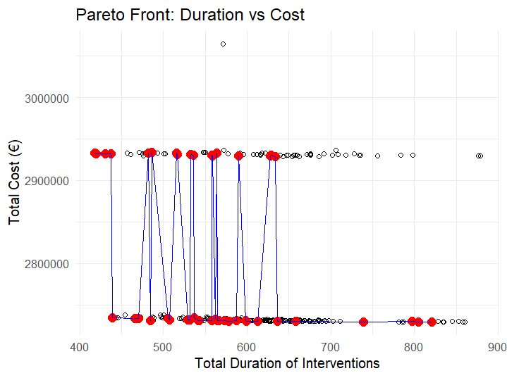
Generations: 60, Population Size: 600.
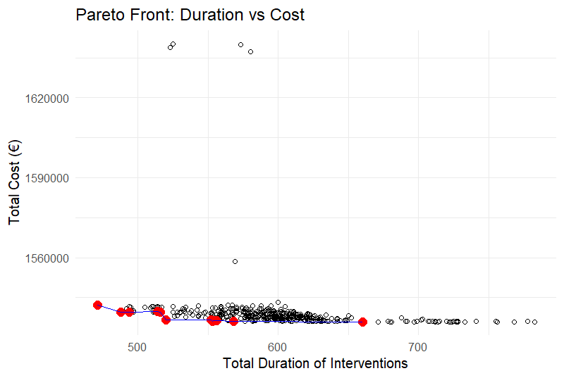
Generations: 70, Population Size: 700.
Strategies selected as best performing
The following analysis presents the strategies that perform best across general costs, including both environmental and material expenditure, as well as total interruption duration. Table 2 below outlines the specific maintenance intervals for each system, highlighting the interventions where the frequency difference between strategies exceeds four years, as indicated in bold.
While no specific inference is drawn from these individual shifts, it is evident that the strategy optimised for duration relies on the highest degree of overlapped interventions to reduce on-site activity.
| Frequency Ranges | Pareto Optimised Strategies by Criteria | |||||
| System | Intervention | Min. | Max. | Cost / Env. | D. Duration | Selected |
| Precast Concrete Facade | Coating Refresh | 12 | 18 | 18 | 16 | 18 |
| Joint Maintenance | 15 | 25 | 25 | 20 | 20 | |
| Panel Replacement* | 40 | 60 | 60 | 60 | 60 | |
| Glass Curtain Wall | Deep cleaning | 5 | 10 | 10 | 8 | 10 |
| gasket replacement | 8 | 14 | 14 | 8 | 12 | |
| IGU replacement* | 40 | 60 | 60 | 60 | 60 | |
| Steel Truss Bridge | Member Replacement | 50 | 70 | 62 | 66 | 60 |
| Full Recoating* | 20 | 30 | 30 | 20 | 20 | |
| Building Reinforced | Spall Repair | 15 | 25 | 25 | 20 | 18 |
| Crack Sealing / Joints Refurbishment* | 30 | 50 | 40 | 30 | 40 | |
| Carbonation Treatment | 3 | 7 | 20 | 20 | 20 | |
| Structural Grounding | 10 | 20 | 30 | 30 | 30 | |
| Railway Track Concrete Sleepers | Systematic sleeper renewal campaign | 40 | 60 | 60 | 60 | 60 |
| Full Rail Renewal* | 60 | 100 | 70 | 61 | 64 | |
| Railway Track Timber Sleepers | Full sleeper renewal | 15 | 30 | 30 | 30 | 30 |
| Geotextile full replacement | 80 | 120 | 120 | 120 | 120 | |
| Full Rail Renewal | 60 | 100 | 60 | 60 | 60 | |
*High emission contributing intervention (in comparison with the other present in the integrated system)
Table 3 presents the LCA results for these strategies, illustrating the clear trade-off between financial expenditure and system downtime. The selected strategy provides a balanced middle ground, reducing duration significantly compared to the cost-optimised version while maintaining lower total costs than the duration-optimised extreme.
| Pareto Optimised Strategies by Criteria | |||
| Performance Indicator | Cost | Downtime Duration | Selected |
| Duration | 660 | 471 | 494 |
| Energy | 14.457.841 | 14.484.433 | 14.483.846 |
| CO2 | 1.020.997 | 1.022.614 | 1.022.232 |
| NOx | 2.373 | 2.374 | 2.373 |
| Cost | 1.535.927 | 1.542.049 | 1.539.428 |
| Total Costs | 2.998.637 | 3.007.375 | 3.004.540 |
Scalability
Finally, it is essential to consider the institutional context of railway management. While this analysis utilised a 1 km reference section, railways are typically managed as vast, integrated networks. The frequency of high-impact interventions, such as full railway renewal, proved highly sensitive to the defined system lifetime. At the current reference scale, such renewals occur only once; however, as the analysed lifetime or physical track length increases, the frequency and subsequent financial impact of these interventions would likely shift. For decision-makers, this highlights the need to scale these localised findings to broader institutional frameworks to fully capture the lifecycle dynamics of the network.