Optimization Setup and Algorithm:
The multi-objective optimization was implemented using the NSGA-II evolutionary algorithm, as explicitly defined in the optimization code. The algorithm was selected for its ability to handle high-dimensional decision spaces and conflicting objectives.
The optimization was executed with 20 generations and a population size of 100. A fixed random seed (123) was used to ensure reproducibility of results.
Decision Variables and Bounds:
The optimization considers 14 decision variables corresponding directly to maintenance intervention frequencies and geometric parameters defined in the system intervention dataset.
| Index | Subsystem | Symbol | Description | Bounds |
| 1–4 | Road | M, MS, SDO, DR | Road maintenance intervention intervals (years) | 3–40 |
| 5–6 | DN300 Sewer | PPR3, PRP3 | Partial pipe repair / replacement intervals (years) | 30–80 |
| 7–8 | DN200 Water | PPR, IEPR | Repair and lining intervals (years) | 60–100 |
| 9–11 | Manholes | MLR, REH, RPL | Repair / rehabilitation / replacement intervals (years) | 15–80 |
| 12 | Road geometry | Road width | Excavation width (m) | 8–15 |
| 13 | Road geometry | Asphalt thickness | Pavement thickness (m) | 0.08–0.15 |
| 14 | Manhole geometry | Manhole diameter | Manhole internal diameter (m) | 0.9–1.1 |
Structure of Pareto-Optimal Solutions:
A parallel coordinate plot was used to examine how Pareto-optimal solutions are distributed across the decision space and objective dimensions.
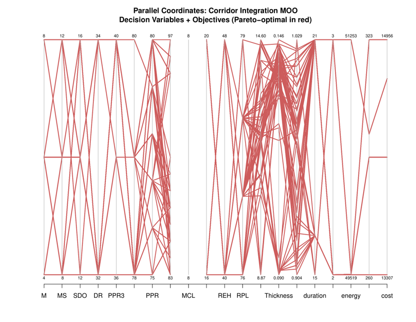
Figure 01: Parallel coordinate plot showing decision variables and objective outcomes for Pareto-optimal corridor maintenance strategies.
The dispersion of Pareto-optimal solutions across most decision variables indicates that no single intervention frequency or geometric parameter dominates system performance. This reflects strong coupling between objectives and the discrete nature of intervention schedules.
Objective-Space Trade-Offs
An objective-space projection was used to visualize trade-offs between intervention duration and environmental performance.
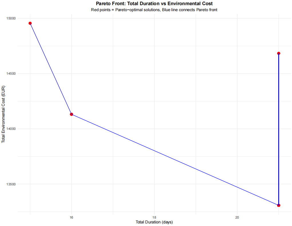
Figure 02: Pareto front illustrating the trade-off between total intervention duration and total environmental cost.
Interpretation and Limitations:
The multi-objective optimization identifies a set of equivalently efficient maintenance strategies rather than a single optimal solution. The results highlight both the flexibility of coordinated maintenance and the limitations of the current formulation.
Clarification on optimization inputs and bounds: The multi-objective optimization is defined over a 14-dimensional decision space, where each dimension corresponds to an individual maintenance intervention or geometric parameter. Each intervention variable has its own independently defined lower and upper bounds. Variables are grouped by subsystem only for readability and have no influence on the optimization itself.
The intervention bounds do not represent physical failure limits. Instead, they define the allowable search range for each intervention interval. Lower bounds correspond to very frequent but still engineering-reasonable maintenance, while upper bounds represent delayed interventions that are still considered acceptable. These bounds are modelling assumptions appropriate for exploratory system-level analysis and are not intended to be unique or definitive.