Multi-Objective Optimization – Virtual City Model

Introduction

In this study, the service level of the integrated system is defined in terms of system availability over the 25-year analysis horizon. System availability is quantified through the total duration of maintenance-related interruptions, which represents the cumulative time during which the integrated system is not fully operational. As all subsystems are functionally coupled, maintenance interventions on individual components reduce the service level of the system as a whole. Minimizing total intervention duration therefore directly corresponds to maximizing the system service level. Based on this definition, the objective of multi-objective optimization is to identify efficient maintenance strategies for the integrated infrastructure system by explicitly balancing competing performance criteria. Rather than searching for a single “optimal” solution, the analysis investigates how trade-offs emerge between maintenance performance (service level), environmental impacts, and economic costs across the solution space.

Each maintenance strategy is defined by a specific combination of intervention frequencies, intervention durations, and coordination patterns across subsystems. For every strategy, system-level performance is evaluated over the unified 25-year analysis horizon using a consistent set of indicators:

Duration
Intervention distance
CO2 emissions
NOx emissions
SO2 emissions
Energy
Cost

Together, these indicators form a multi-dimensional objective space in which no single strategy can simultaneously minimize all criteria.

Pareto Optimality and Filtering

All generated strategies are therefore evaluated using a Pareto dominance criterion. A strategy is considered Pareto-optimal if none of its objectives can be improved without worsening at least one other objective. The resulting Pareto front represents the set of most efficient trade-offs between maintenance effort, environmental impact, and cost within the integrated system.

A comparison, shown in Fig. 1, between the objective ranges of all sampled solutions and the Pareto-optimal subset shows that Pareto filtering effectively constrains the solution space, particularly by removing high-cost and high-impact configurations.

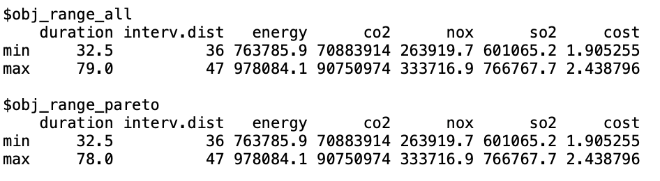
Fig. 1

Specifically, the minimum values for indicators such as duration and intervention distance remain unchanged after filtering. This suggests that the optimal downtime strategies were already captured in the initial sampling; the filtering primarily serves to compress the upper bounds by eliminating “costly and high-polluting” redundant configurations to optimize the system boundary.

Duration-Cost Trade-offs

Building on this reduced solution space, the trade-off structure between maintenance duration and cost is examined using a Pareto front projection, shown in Fig. 2.

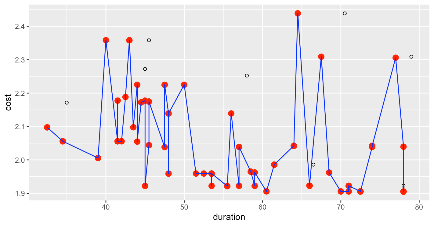
Fig. 2

The Pareto plot illustrates the relationship between total maintenance duration and cost. Rather than exhibiting a clear monotonic trade-off, the Pareto-optimal solutions are distributed across the duration range, with cost-efficient solutions appearing at multiple durations.

Notably, several local regions show comparatively low costs without extreme intervention durations(e.g., around the 45-55 and 70-75 duration marks), suggesting the existence of alternative compromise solutions rather than a single optimal balance point. These solutions highlight that practical trade-offs depend on the joint configuration of maintenance parameters rather than on duration alone.

The Accumulated Impact of Input Parameters

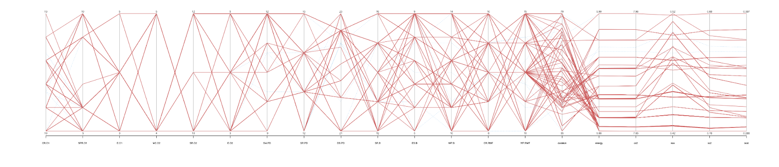
Fig. 3

Fig. 3 presents a parallel coordinate plot of the sampled maintenance strategies and their corresponding system-level performance indicators. Each polyline represents one complete maintenance strategy across all subsystems, spanning decision variables, cumulative duration, and environmental and economic objectives.

Pareto-optimal solutions, highlighted in red, are distributed across a wide range of individual maintenance parameters, indicating that no single decision variable dominates the optimization outcome. Instead, Pareto performance emerges from coordinated combinations of maintenance actions across subsystems.

While individual maintenance parameters exhibit high variability, Pareto-optimal solutions show partial convergence in cumulative duration, suggesting that system-level downtime acts as a mediating constraint without fully determining environmental or cost performance. On the objective axes, trade-offs between energy use, emissions, and cost remain visible within the Pareto subset, confirming the multi-objective nature of the optimization problem

To account for the large magnitude differences between environmental indicators and decision variables, objective values were log-transformed for visualization, improving readability while preserving Pareto dominance.

Scenario Development

From the Pareto-optimal solution set, four representative maintenance scenarios were selected for detailed comparison.

These scenarios were not obtained through additional optimization runs, but through post-processing of the Pareto front in order to illustrate distinct trade-off patterns.

Scenario A min Duration

The first scenario corresponds to the solution with the minimum total intervention duration, representing the highest system service level. By clustering maintenance activities and improving coordination across subsystems, this schedule minimizes overall downtime and reduces the frequency of service interruptions.

Compared with baseline maintenance planning, the total duration is significantly reduced, indicating that integrated scheduling can effectively enhance system availability. This scenario is particularly recommended for infrastructure systems where operational continuity is critical, such as energy supply and commercial facilities, since shorter interruptions help maintain stable services and reduce disruption to users.

Scenario B min Emission(CO2, SO2, NOx) and Costs

The second scenario represents the strategy that simultaneously achieves the lowest environmental emissions and total cost within the Pareto-optimal set. This outcome is primarily driven by longer maintenance intervals and fewer large-scale interventions, which reduce material consumption, energy use, and associated emissions.

Although this strategy results in a longer cumulative maintenance duration, it provides clear advantages from both environmental and economic perspectives. Therefore, it is well suited for decision contexts where sustainability and lifecycle cost efficiency are prioritized over short-term service availability.

Scenario C Max Intervention Distance

The third scenario represents a low-maintenance-intensity regime, selected as the Pareto-optimal solution with the largest intervention spacing (interv.dist).By extending the intervals between maintenance activities, this strategy reduces intervention frequency while maintaining acceptable system performance levels.

Although the total duration (45 days) is higher than that of the minimum-duration scenario, it remains moderate compared to other solutions. Environmental impacts and costs also stay relatively controlled, indicating that longer maintenance intervals do not necessarily lead to disproportionate system burdens.

This scenario is particularly suitable for projects prioritizing operational stability and reduced maintenance disruption. It demonstrates that strategically spacing interventions can balance service continuity with environmental and economic performance without requiring excessively frequent repairs.

Scenario D Balanced Compromise

Scenario D represents a balanced maintenance strategy selected from the Pareto-optimal set to achieve a compromise between system availability, environmental impact, and economic cost. Rather than minimizing a single objective, this scenario maintains moderate performance across all indicators, avoiding extreme trade-offs.

With a total intervention duration of 47.5, the strategy significantly reduces downtime compared to high-duration solutions while remaining more operationally stable than the minimum-duration scenario. At the same time, energy use, emissions, and cost remain within an acceptable mid-range, indicating that improved service continuity is achieved without disproportionately increasing environmental or financial burdens.

This scenario is particularly suitable for long-term infrastructure management where decision-makers must balance reliability with sustainability. By distributing maintenance activities more evenly over time and preventing excessive intervention clustering, the strategy supports predictable system operation while maintaining overall efficiency.

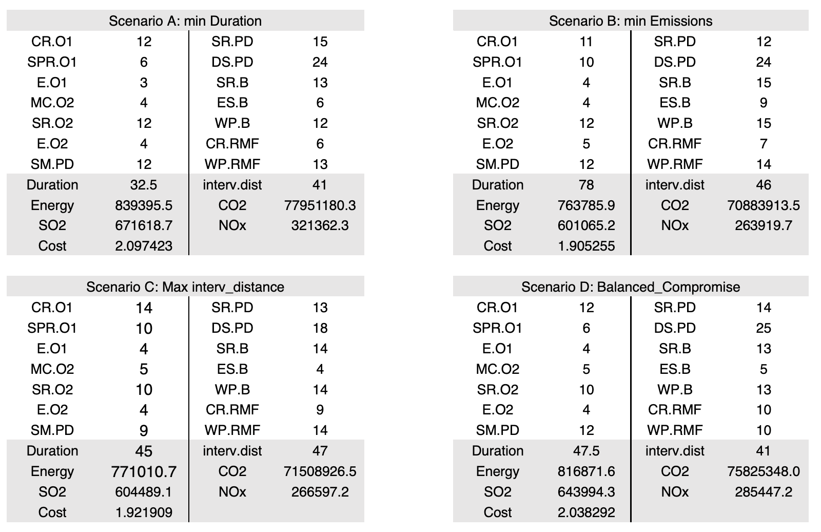
Together, these four scenarios provide a representative overview of the solution space and enable a qualitative comparison of different maintenance planning priorities.

References

Ostermeyer, Y., Wallbaum, H., & Reuter, F. (2013). Multidimensional Pareto optimization as an approach for site-specific building refurbishment solutions applicable for life cycle sustainability assessment. The International Journal of Life Cycle Assessment, 18(9), 1762–1779. https://doi.org/10.1007/s11367-013-0548-6

Pombo, O., Allacker, K., Rivela, B., & Neila, J. (2016). Sustainability assessment of energy saving measures: A multi-criteria approach for residential buildings retrofitting—A case study of the Spanish housing stock. Energy and Buildings, 116, 384–394. https://doi.org/10.1016/j.enbuild.2016.01.019

Azapagic, A., & Clift, R. (1999). The application of life cycle assessment to process optimisation. Computers & Chemical Engineering, 23(10), 1509–1526. https://doi.org/10.1016/S0098-1354(99)00308-7