1. Scenario Exploration Framework and Parameter Ranges
To explore more maintenance strategies, we conducted a scenario exploration using an n.grid value of 2 (When n.grid > 2, the model runtime increases significantly; therefore, it should be set to 2 for better efficiency.) to control the design space for the exploration. The following are the ranges for intervention events, and more scenarios can be explored through an automated process:
- Highway
3 >= M_h <= 8
10 >= R_h <= 25
20 >=O_h <= 40
- Urban Road
2 >= M_u <= 9
10 >= R_u <= 25
20 >=U_u <= 40
- Drainage
4 >= C_d <= 9
20 >= R_d <= 40
2. Result
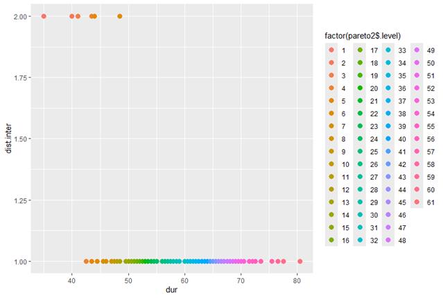
The results are shown in Figure 9, which demonstrates the relationship between dist.inter (the interval between interventions) and dur (total maintenance duration).
This figure reveals the distribution of intervention frequency and total maintenance time. Most points in the graph are concentrated around lower dist.inter values, indicating that in these scenarios, the intervals between interventions are shorter. A total of 61 maintenance strategies were derived, with each point representing a unique strategy.
As shown in Figure 9, based on the differences in intervention intervals and total duration (from bottom to top), these strategies can be divided into two categories:
- Short Interval, Long Total Duration (dist.inter = 1.0, dur 42-82): Intervention frequency is extremely high, with very short intervals between interventions. The total maintenance duration can vary significantly. This maintenance strategy is applicable to independent subsystems where maintenance activities are conducted separately.
- Long Interval, Short Total Duration (dist.inter = 2.0, dur 35-50): Intervention frequency is the lowest, while the total maintenance duration remains under 50 days. This suggests a quick but less frequent intervention, minimizing downtime. This is suitable for systems where subsystems are tightly interconnected.
However, due to the similar color scheme of the optimal solutions, it is difficult to visually identify them. Therefore, we will use the Pareto frontier to highlight the optimal solutions.
3. Pareto frontier
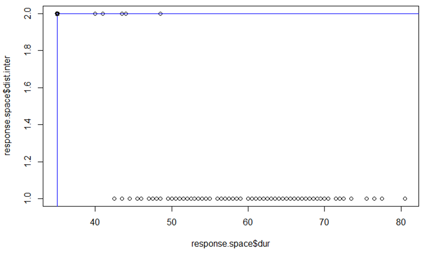
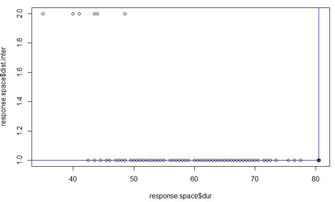
Figures 10 and 11 illustrate the Pareto front, from which we can easily identify the optimal solution. The blue line represents the Pareto front. The optimal solution with the shortest total duration and longest event interval is located at the black dot in the upper left corner, while the optimal solution with a longer maintenance time and shorter event interval is located at the black dot in the lower right corner. These solutions represent different strategies, which can help us further perform multi-objective optimization. For example, if I need the strategy with the shortest total duration, I would choose the strategy in the upper left corner. Therefore, we can use this method to select the optimal maintenance strategy according to our needs according to our needs.
4. Conclusion
Based on the charts and data, the following conclusions can be drawn:
- The reduction in total downtime indicates that this maintenance plan can effectively reduce system downtime and improve resource utilization.
- The relationship between maintenance intervals and total duration helps us choose different maintenance strategies, aiming to minimize downtime while ensuring maintenance frequency.
- The Pareto front demonstrates a comparison between various maintenance strategies, providing a reference for subsequent multi-objective optimization.
References:
- Deb, K., Pratap, A., Agarwal, S., & Meyarivan, T. (2002). A fast and elitist multiobjective genetic algorithm: NSGA-II. IEEE Transactions on Evolutionary Computation, 6(2), 182–197.
- Hakanen, J., Sahlstedt, K., & Miettinen, K. (2021). Multiobjective optimization and decision making in engineering design. Optimization and Engineering.
- Ehrgott, M., et al. (2025). Fifty years of multi-objective optimization and decision making: A survey. European Journal of Operational Research.
- Pourgholamali, M., et al. (2023). Multi-objective optimization in highway pavement management: A state-of-the-art review. Journal of Road Engineering.
- Santos, J., Bryce, J., Flintsch, G., Ferreira, A., & Diefenderfer, B. (2017). A multi-objective optimization-based pavement management decision support system. Journal of Cleaner Production, 164, 1380–1393.
- Harvey, M. O. (2012). Optimising Road Maintenance. International Transport Forum (OECD), Discussion Paper 2012-12.
- Wang, Z., et al. (2017). Application and analysis of methods for selecting an optimal solution from the Pareto-optimal front. Industrial & Engineering Chemistry Research, 56(1), 232–246.
- Owa, A. (2019). Multi-Objective Optimization for Time-based Preventive Maintenance Planning (PhD thesis). Nottingham Trent University.