For Strategy 4, material inventories and associated environmental indicators are defined with explicit consideration of the structural role of each subsystem. Data are sourced from established literature and widely used life-cycle databases, but their application within the assessment reflects a hierarchical system of interpretation rather than uniform treatment across components. Material quantities are expressed per functional unit appropriate to each subsystem (per cubic meter or per square meter), ensuring consistency while preserving subsystem-specific characteristics.
The NSGA-II Pareto front illustrates how total system interruption duration and total life-cycle cost interact under Strategy 4 when structural-safety constraints dominate maintenance planning. In figure 4.c each point in the plot represents a complete, feasible integrated maintenance plan over the 100-year service life that satisfies all technical constraints, including fixed maintenance schedules for the gravity and cantilever retaining walls and limited flexibility for non-critical subsystems. The horizontal axis shows the cumulative interruption duration in days, meaning the total number of days during which the system experiences reduced functionality due to maintenance activities across all subsystems; values closer to the left indicate solutions with less overall disruption, while values further to the right correspond to solutions where maintenance activities extend over more days in total. The vertical axis shows the total life-cycle cost in euros, aggregating material costs, execution costs, and intervention-related expenses for all maintenance actions; lower points therefore represent more cost-efficient strategies, whereas higher points indicate solutions with greater financial demand, often due to more frequent, more intensive, or less efficiently sequenced interventions.
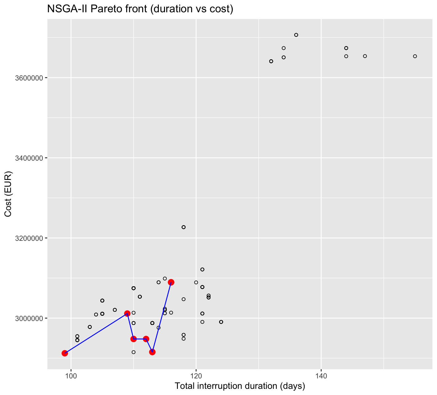
It shows that almost all feasible solutions for Strategy 4 are concentrated within a narrow interruption range between roughly 100 and 120 days on the x-axis, while costs on the y-axis vary much more widely, from approximately 2.95 million EUR up to about 3.7 million EUR. This horizontal concentration is a direct consequence of the structural-safety-driven logic of Strategy 4: the gravity and cantilever retaining walls have fixed, non-adjustable maintenance schedules that repeatedly trigger system-level interventions, effectively locking the cumulative interruption duration into a tight band. As a result, even when non critical subsystems are shifted within their allowable ranges, they can only marginally increase or decrease total interruption duration, explaining why solutions do not extend far below 100 days or above 120 days. Within this constrained x-range, differences between solutions are expressed primarily in cost, not duration. For example, at interruption durations close to 100–105 days, costs cluster around 2.95–3.05 million EUR, representing solutions where non-critical subsystem maintenance is arranged with minimal additional execution effort around the fixed retaining-wall interventions. Moving toward 110–115 days, costs increase to around 3.05–3.15 million EUR, indicating configurations where maintenance actions are less efficiently aligned, leading to higher execution or material expenses even though the overall disruption level changes only slightly. Beyond 120 days, a small number of solutions exhibit substantially higher costs—exceeding 3.6 million EUR—without a meaningful reduction or increase in interruption duration, which makes them clearly inferior from a system-level perspective.
The fact that points are densely packed horizontally but spread vertically confirms that, under Strategy 4, interruption duration is largely structurally constrained, while cost remains the primary differentiating outcome. Points that are very close together on the x-axis but far apart on the y-axis represent maintenance plans with nearly identical system availability performance but significantly different economic consequences, often driven by how non-critical repairs, replacements, or rehabilitation actions are sequenced relative to the fixed retaining-wall schedule. This explains why the Pareto front does not exhibit a smooth diagonal trend but instead appears almost vertical: the optimization cannot trade large reductions in interruption duration for cost, because spacing and frequency are dictated by structural maintenance needs. In summary, the graph shows that Strategy 4 offers limited flexibility in reducing disruption, with most viable solutions constrained to the 100–120-day range, and that decision-making therefore centers on selecting cost-efficient solutions within this structurally imposed interruption window rather than attempting to reshape the timing behavior of the system.
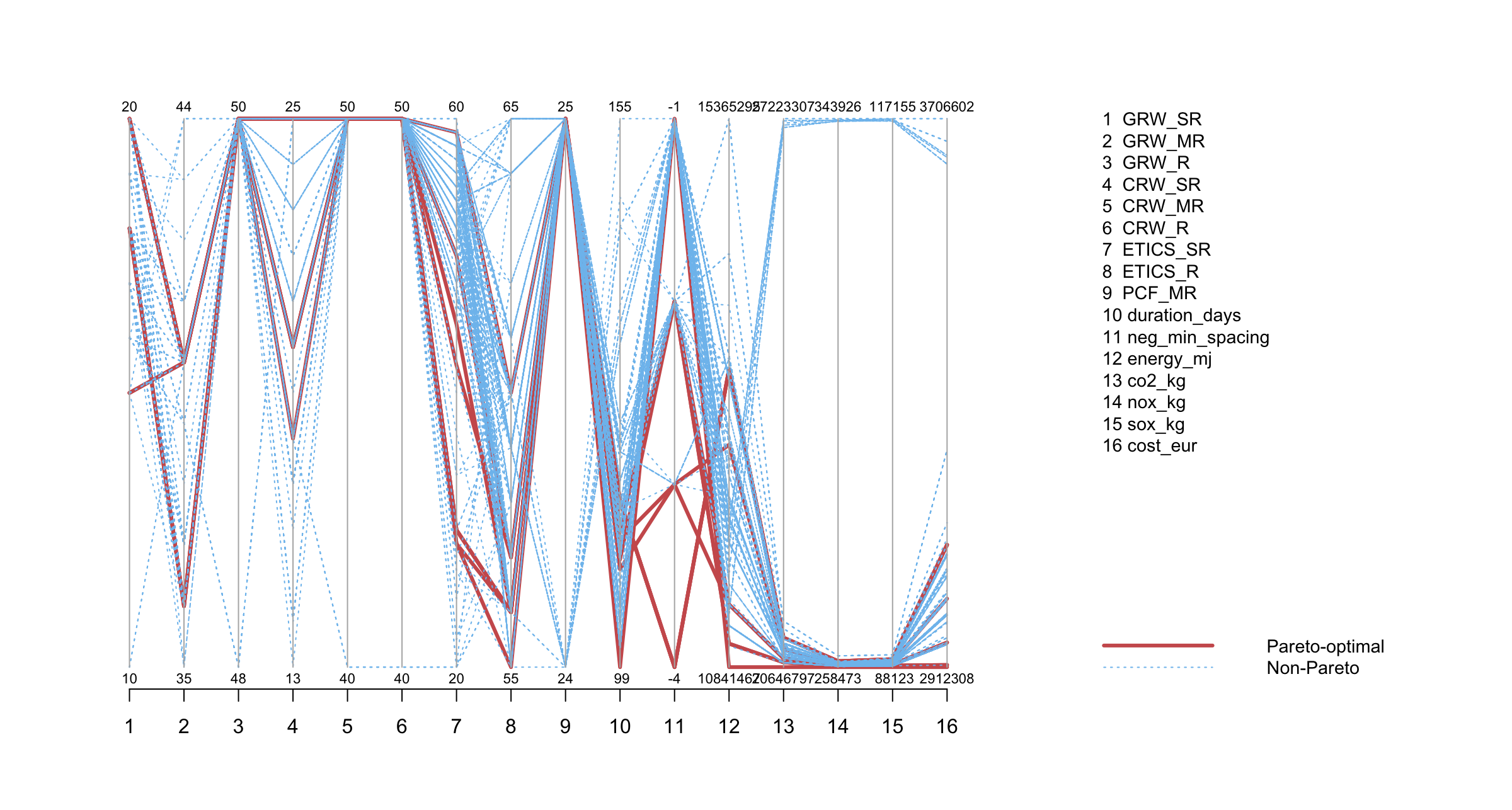
This parallel-coordinates plot (figure 4.d) provides a comprehensive system-level view of how individual maintenance decisions, environmental indicators, and economic outcomes interact for Strategy 4, distinguishing clearly between Pareto-optimal solutions (solid red lines) and non-Pareto solutions (dashed blue lines). Each vertical axis represents one decision variable or outcome, ordered from left to right: maintenance actions for the gravity retaining wall (GRW_SR, GRW_MR, GRW_R), cantilever retaining wall (CRW_SR, CRW_MR, CRW_R), ETICS (ETICS_SR, ETICS_R), PCF major repair (PCF_MR), followed by performance indicators including total interruption duration in days, minimum spacing between interventions in years, energy demand (MJ), emissions (CO₂, NOx, SOx in kg), and total life-cycle cost in euros. The numerical ranges shown at the top and bottom of each axis indicate the admissible or observed bounds for each variable, allowing direct comparison of how different solutions populate the feasible space.
A key observation from the figure is that Pareto-optimal solutions occupy a much narrower band across the first nine axes, which correspond to retaining wall and major structural maintenance actions. This reflects the core logic of Strategy 4: maintenance schedules for the gravity and cantilever retaining walls are largely fixed and non-negotiable, resulting in limited variability for these parameters across all feasible solutions. In contrast, non-Pareto solutions exhibit greater dispersion in these axes, indicating that deviations from the fixed structural maintenance logic tend to degrade overall performance. Moving to the duration_days axis, both Pareto and non-Pareto solutions cluster tightly around values close to 100 120 days, confirming what was observed in the Pareto front: total interruption duration is structurally constrained by recurring retaining wall interventions and cannot be significantly reduced or increased through integration. The energy_min_spacing axis shows similarly limited variation, reinforcing that spacing is governed by safety-critical components rather than by optimization of freedom.
The distinction between Pareto-optimal and non-Pareto solutions becomes much more pronounced in the environmental and economic outcome axes. While energy demand and emissions (CO₂, NOx, SOx) span wide numerical ranges—visible in the strong vertical spread of lines—Pareto-optimal solutions consistently occupy the lower portions of these axes, indicating reduced environmental impact for a given interruption regime. The same pattern is especially clear in the cost_eur axis, where Pareto-optimal solutions cluster near the lower end of the cost range (approximately 2.9–3.1 million EUR), whereas non Pareto solutions extend upward toward significantly higher costs without any corresponding benefit in interruption duration or spacing. Lines that cross sharply upward in the cost and emissions of axes while remaining similar elsewhere represent dominated solutions: they are more expensive and environmentally intensive while offering no improvement in system availability.
Overall, the figure shows that under Strategy 4, optimality is achieved not by altering structural maintenance decisions or system timing, but by controlling the environmental and cost consequences of non-critical subsystem interventions within a structurally fixed framework. The parallel-coordinates representation makes this explicit by showing that Pareto-optimal solutions are characterized by alignment and consistency across all axes, particularly in the outcome dimensions, whereas non-Pareto solutions display erratic crossings and higher dispersion. This confirms that Strategy 4 produces a constraint-dominated solution space, where structural safety defines the feasible envelope and optimization operates primarily by minimizing cost and environmental impact within that envelope rather than reshaping maintenance timing or spacing.
Home | System Definition | Scenario 1 | Scenario 2 | Scenario 3 | Scenario 4 | Discussion | Appendix