The scenarios evaluated for the lifecycle assessment and cost analysis were selected from the Pareto optimal solution set identified in the previous step based on service interruption and maintenance spacing criteria, graph shown in figure 1.c . These scenarios were chosen to represent different regions of the Pareto front, with the aim of comparing operational and economic trade-offs at the system level.
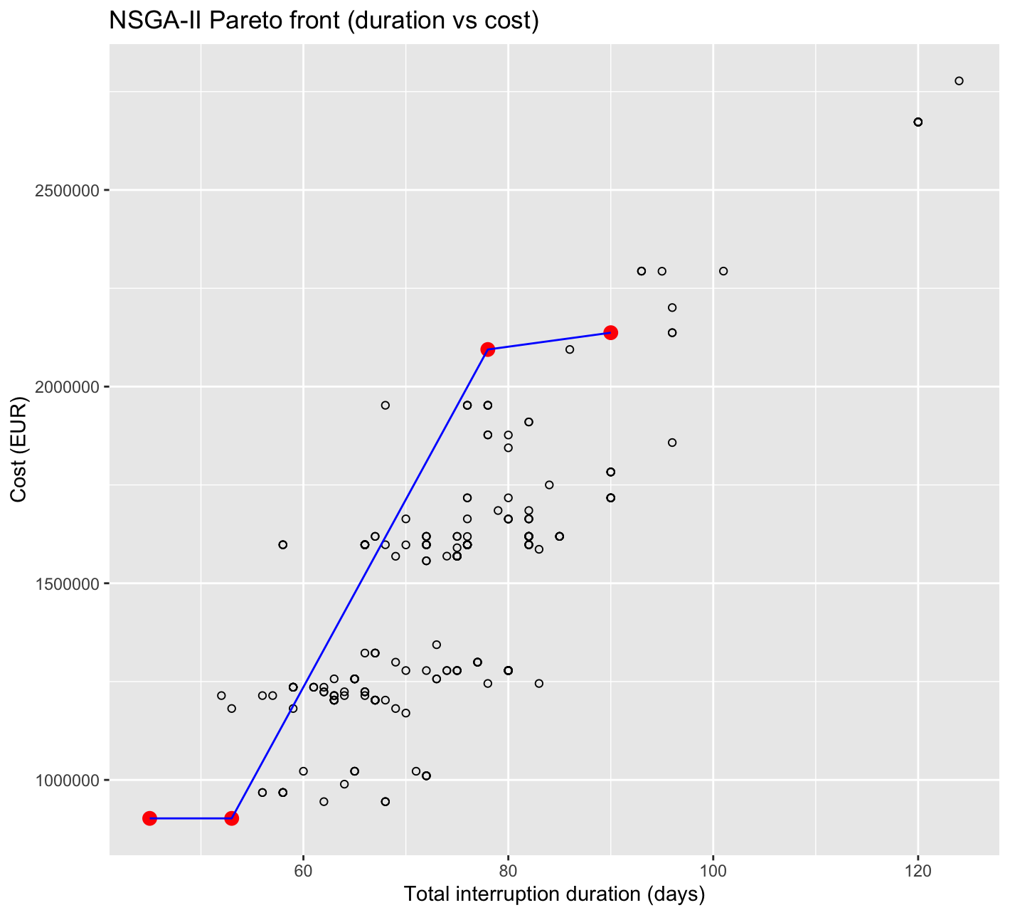
When the overall trend of the graph is examined, it can be observed that within the solution space, increasing total system interruption is associated with increasing costs. This result appears partly surprising and partly intuitive at first glance. Under normal circumstances, one would expect that reducing the level of system interruption would require additional costs. However, the results presented in this graph initially suggest a relationship that contradicts this common expectation.
From personal perspective, it becomes clear that a higher number of maintenance interventions and more frequent interventions represent an important factor contributing to an increase in total interruption duration. In this case, exposing the system to more maintenance activities throughout its life cycle naturally leads to higher overall system costs. From this point of view, the obtained results can be considered internally consistent.
From an engineering perspective, the solution that exhibits both the lowest number of interruption days and the lowest cost appears to be the most attractive option at first glance, creating the impression that no clear trade-off exists between these two objectives. However, this observation strongly depends on the type of maintenance actions on which the maintenance plan is based. When evaluated within the context of the defined maintenance strategy, this solution can be regarded as a reasonable and feasible alternative for the system.
A more detailed examination of the graph reveals a distinct change in behavior along the Pareto front in the range of approximately 60–80 days, where a clear knee point and a more linear relationship emerge. Outside this range, the relationship between system interruption and cost is relatively weak, whereas within this interval, the two variables are clearly and directly related. In other words, up to this point, meaningful reductions in service interruption can be achieved with relatively limited cost increases, while beyond this range, cost increases become significantly more pronounced.
The parallel coordinates diagram in figure 1.d is used to visualize the behavior of integrated
maintenance scenarios within a multicriteria decision space. In the diagram, each vertical axis represents
a parameter or performance indicator considered in the maintenance planning process, while each line
corresponds to a single maintenance alternative. The red lines indicate Pareto-optimal scenarios,
whereas the blue dashed lines represent non-Pareto solutions.
The first ten axes correspond to maintenance related variables associated with the four main system components, while the remaining seven axes represent operational, environmental, and economic performance indicators used in the evaluation.
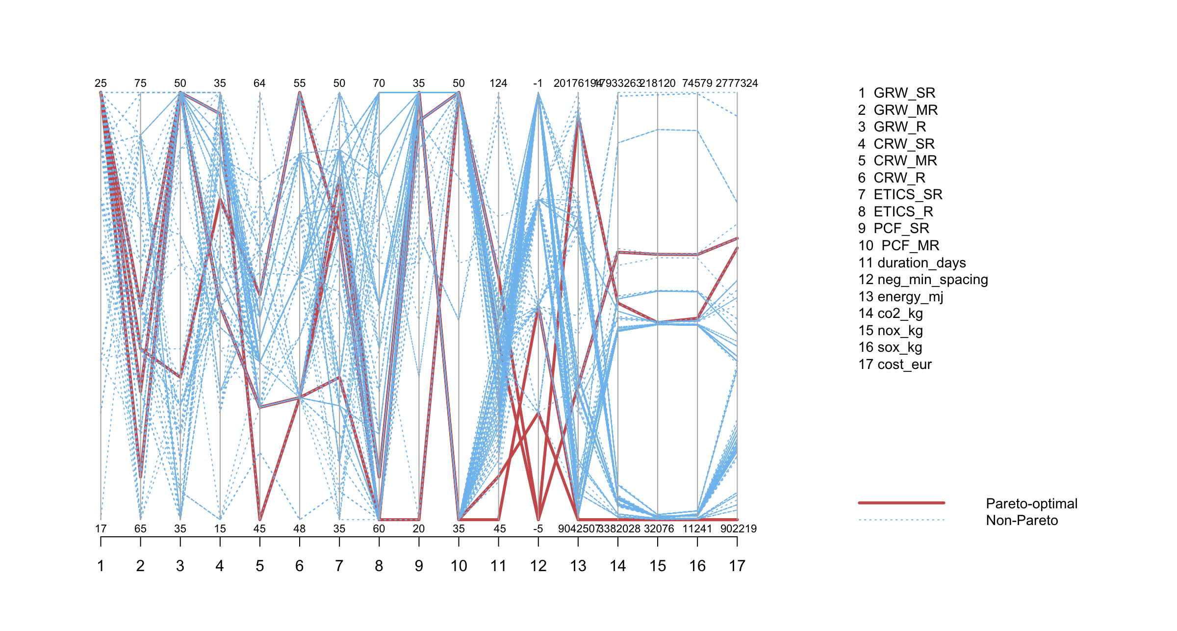
When the graph is examined, it becomes clear that the maintenance frequencies of the gravity type retaining wall show a pronounced tendency toward balance. In particular, across four Pareto optimal alternatives, the maintenance decisions for this subsystem exhibit a similar V-shaped pattern, indicating an effort to remain within the allowable ranges while avoiding extreme values as much as possible. In contrast, the maintenance frequencies of the other system components largely remain close to average values and do not display comparable extreme behavior. This observation suggests that the identified alternatives do not overemphasize a single subsystem but instead provide more balanced and practically feasible system level scenarios. When one subsystem approaches extreme values, other maintenance variables tend to compensate for this effect, preventing excessive deviation at the system level. This balanced behavior is also reflected in the life cycle assessment results, where the consistent and average trends observed in the LCA outputs indicate that this maintenance balance directly influences environmental and economic performance.
While most maintenance related outputs cluster around average values, one alternative stands out by achieving the best overall performance in terms of energy, emissions, and cost simultaneously. An examination of its maintenance frequencies shows that this alternative does not rely on either the most frequent or the least frequent interventions. This indicates that the observed performance cannot be explained by maintenance frequency alone, but rather by more complex system interactions. In this context, a trade-off between intervention duration and material use becomes evident. Some maintenance activities may be completed in shorter time periods but require higher material intensity, while others take longer but result in lower environmental and economic impacts.
When emission indicators are analyzed, noticeable differences between different alternatives can be observed, even though these indicators follow largely parallel trends. At the same time, the total cost values of these alternatives converge to nearly identical levels. This apparent inconsistency can be explained by the fundamentally different ways in which emissions and costs respond to material inventories. As a result, relatively small changes in material composition can lead to clear differences in emission values. In contrast, total cost in this study is driven primarily by the overall quantity of materials rather than their environmental intensity. Consequently, alternatives with similar total material quantities but different material compositions can exhibit comparable costs while producing distinct emission levels.
Another important observation concerns the presence of non-Pareto alternatives that show better performance than Pareto optimal solutions in terms of energy, emissions, or cost. A closer examination of the graph reveals that, despite their advantages in LCA related indicators, these alternatives fail to satisfy key operational performance criteria. In particular, they do not meet the desired targets for total system interruption duration or minimum spacing between maintenance interventions. If the analysis had been limited to LCA results alone, some of these non-Pareto alternatives might have been considered preferable. Their exclusion therefore highlights the importance of evaluating the system as a whole rather than focusing on isolated performance metrics.
Home | System Definition | Scenario 1 | Scenario 2 | Scenario 3 | Scenario 4 | Discussion | Appendix